Contact: John.Salamon@sahmri.com
Abstract
In situ sequencing is a novel method to generate spatially-resolved, in situ RNA localization and expression data, at an almost single-cell resolution. Few methods, however, currently exist to analyze and visualize the complex data produced, which can encode the localization and expression of a million or more individual transcripts in a tissue section. Here, we present InsituNet, an innovative new application that converts in situ sequencing data into interactive network-based vizualizations, where each unique transcript is a node in the network and edges represent the spatial co-expression relationships between transcripts. InsituNet enables the analysis of the relationships that exist between these transcripts and can uncover how spatial co-expression profiles change in different regions of the tissue or across different tissue sections.
InsituNet is a software package for generating network visualizations from spatially-resolved sequencing data. InsituNet combines 2D region selection, network creation, and network comparison via synchronized layouts into a single Cytoscape app, with a focus on speed and ease of use. As a Cytoscape app, InsituNet’s networks can both be exported into many other formats or utilised by other software within the Cytoscape ecosystem.
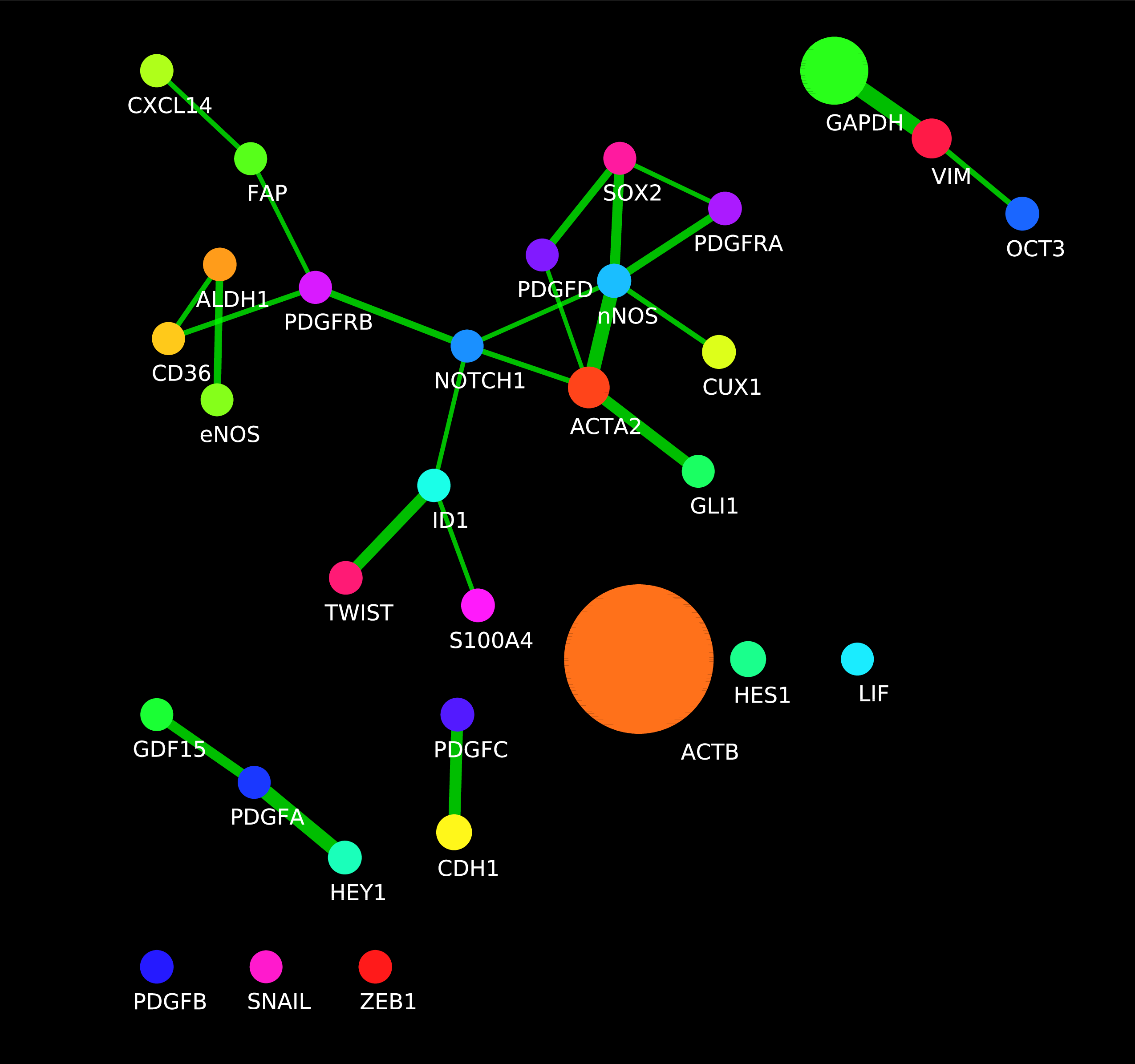
InsituNet’s networks represent spatial co-expression between transcript pairs in an in situ sequencing dataset. Each node represents a specific transcript, and its size is proportional to the abundance of this particular transcript within the tissue section or region selected. Edges by default represent significant spatial co-expression between the two transcripts they link.
Any form of spatially-resolved data in the form of x and y coordinates can be imported for use within InsituNet. Users may select different 2D regions within the dataset to generate networks, and then compare the results in different regions by synchronizing layouts.
The screenshots that appear in this documentation were all taken on macOS 10.12.6, appearance on different platforms is likely to vary slightly.
If you do not already have Java and Cytoscape installed, first download and install the latest versions from https://www.java.com/en/download and http://cytoscape.org. Once complete you may download and install InsituNet manually, or automatically from the Cytoscape app store. For any issues encountered while using Cytoscape not documented here, please consult the Cytoscape manual, available at http://www.cytoscape.org/manual/Cytoscape3_6_0Manual.pdf.
Once Cytoscape is running you can install InsituNet from within the Cytoscape app store, accessible from the top menubar (Apps → App Manager...).
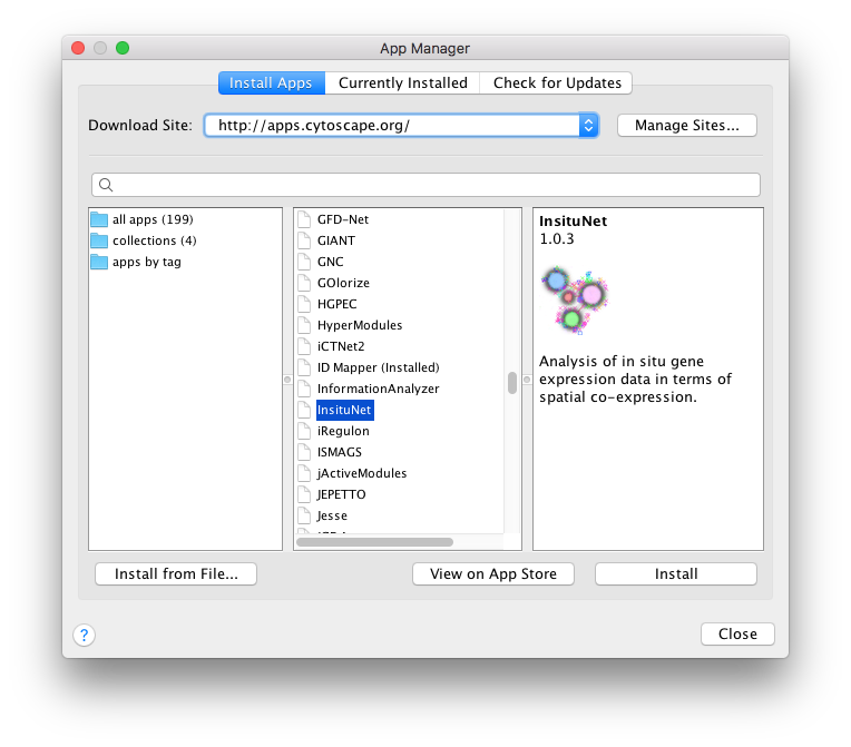
The App Manager window will list available apps from the Cytoscape app store, simply scroll down to or search for “InsituNet” and press the “Install” button. If your computer is behind a proxy you may need to configure Cytoscape proxy settings to access the App store via Edit → Preferences → Proxy settings.
You may install InsituNet by manually downloading it from http://apps.cytoscape.org/apps/insitunet, then selecting Install from File from the App Manager (Figure 1).
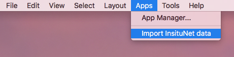
After download and installation is complete, InsituNet can be started by importing a dataset from Apps → Import InsituNet data.
InsituNet takes input in the form of x and y coordinates. This input should be provided in a file of comma separated values. This file must contain at least 3 columns, one for transcript name, and one each for x and y coordinates. The first row is the header row (eg. name, x, y) and each row after this header represents a single transcript. An example part of a file is shown here:
| name, | x, | y |
| ACTB, | 5.04, | 6.35 |
| GAPDH, | 9.66, | 4.13 |
| ACTB, | 7.65, | 2.21 |
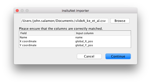
The order of the columns and the exact name of column headers is not important as you will be prompted to check the columns are correct on import. The order of the rows is also irrelevant, so long as the header comes first.
Select the cells under “Input column” to change their value. Once you have verified that the fields of Name, X coordinate and Y coordinate are correctly aligned, press continue. The dataset will be imported, and the main control panel will appear.
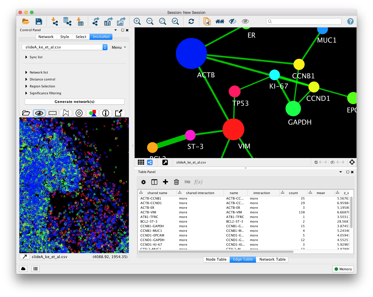
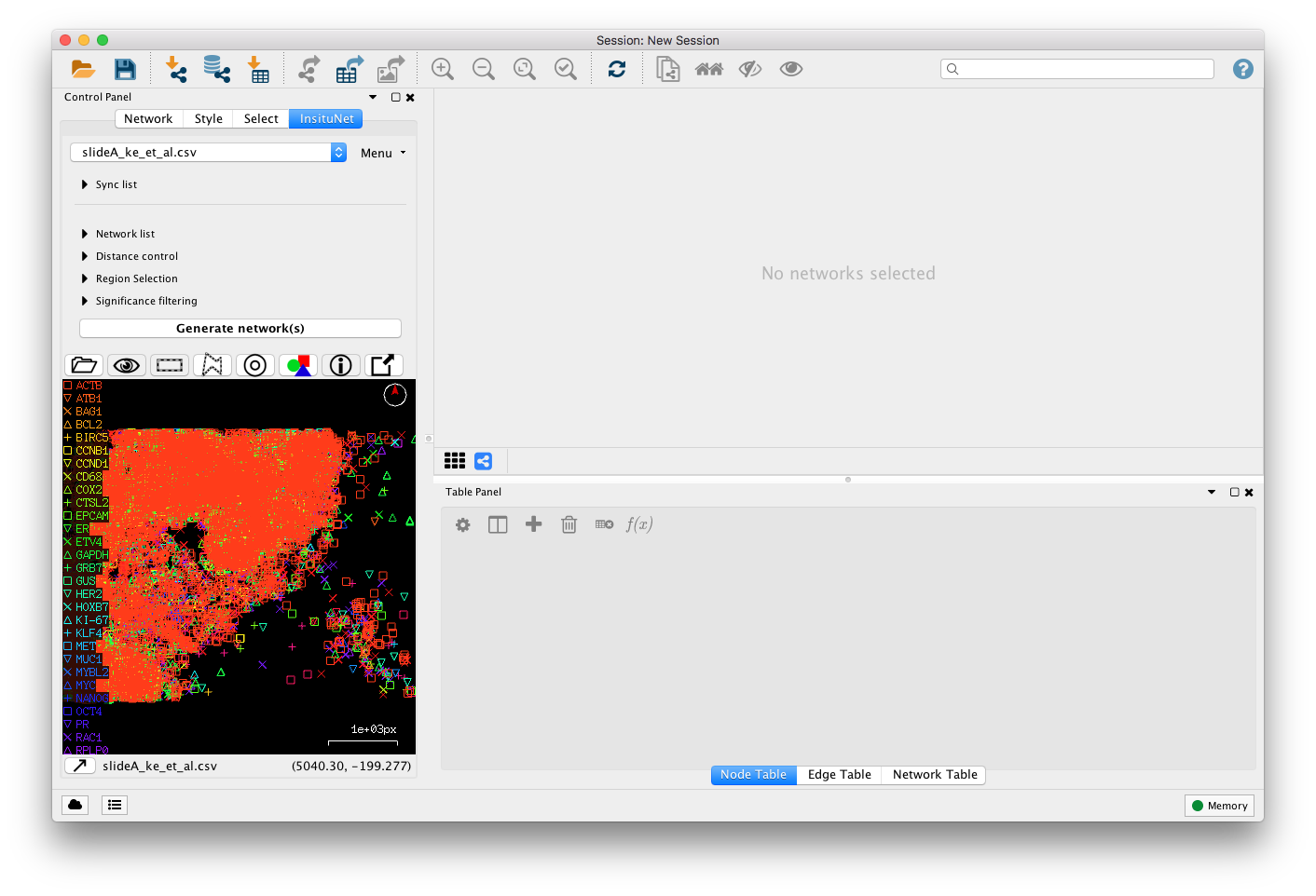
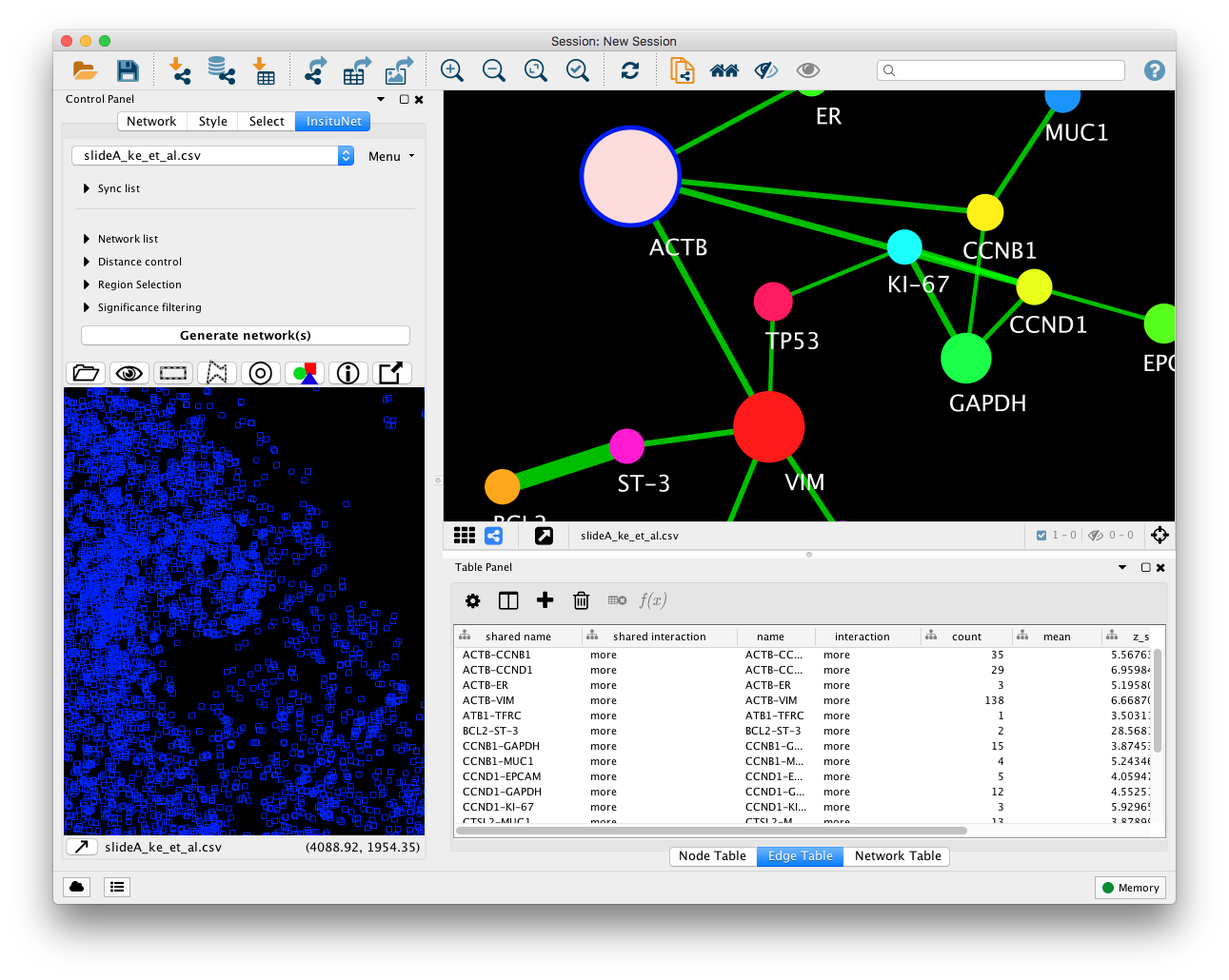
The Insitunet control panel is added as a tab labeled “InsituNet” to the main Cytoscape control panel, which by default is found to the left of the screen. The panel should automatically switch to this tab as seen below just after importing data. Initially, the submenus of the control panel are hidden, but can be expanded by clicking on their titles (network list, distance control, etc.). The name of the currently imported file can be found at the top of the panel. Options to obtain basic information and delete the current dataset are found in the menu directly to the right of this.
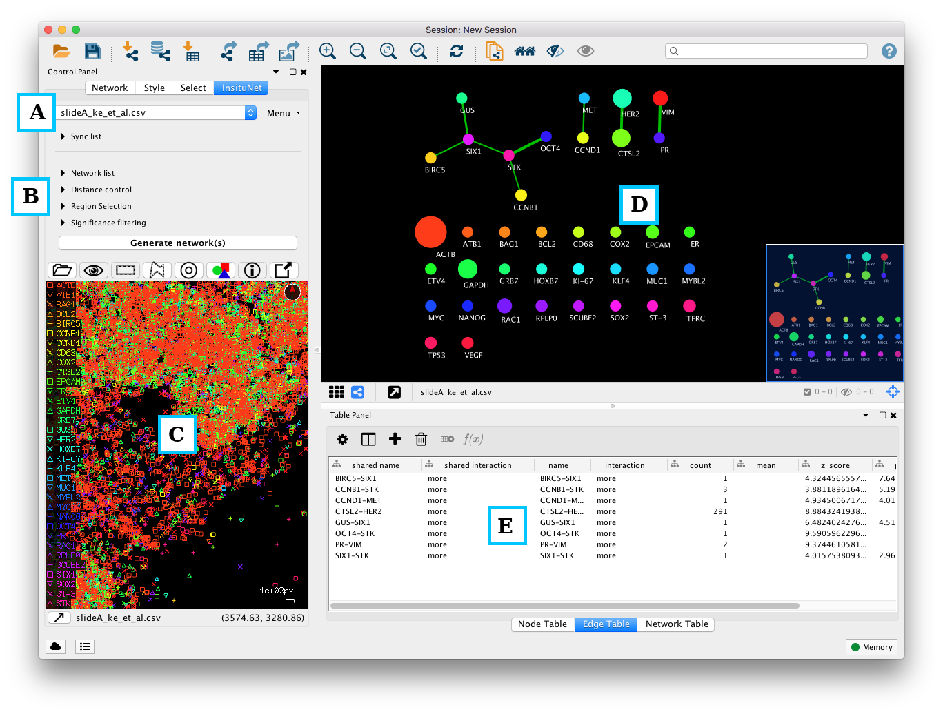
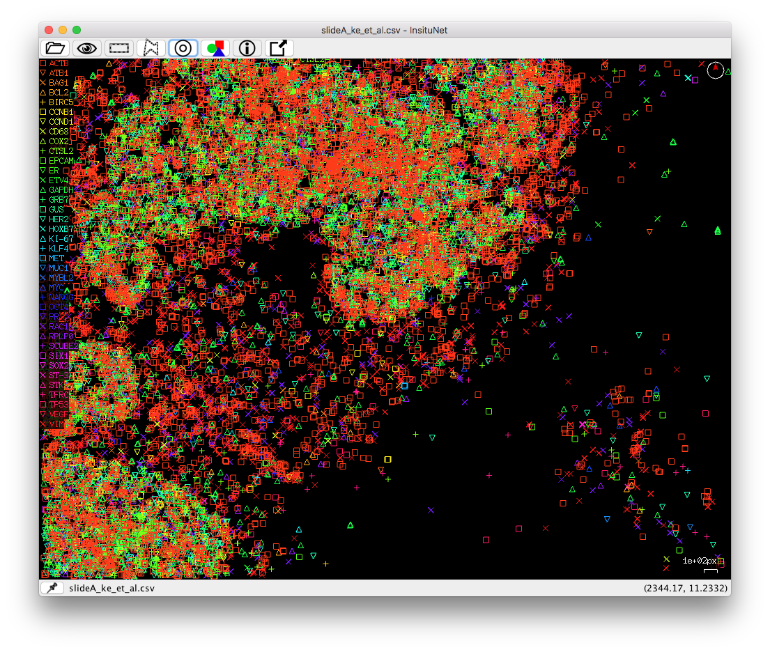
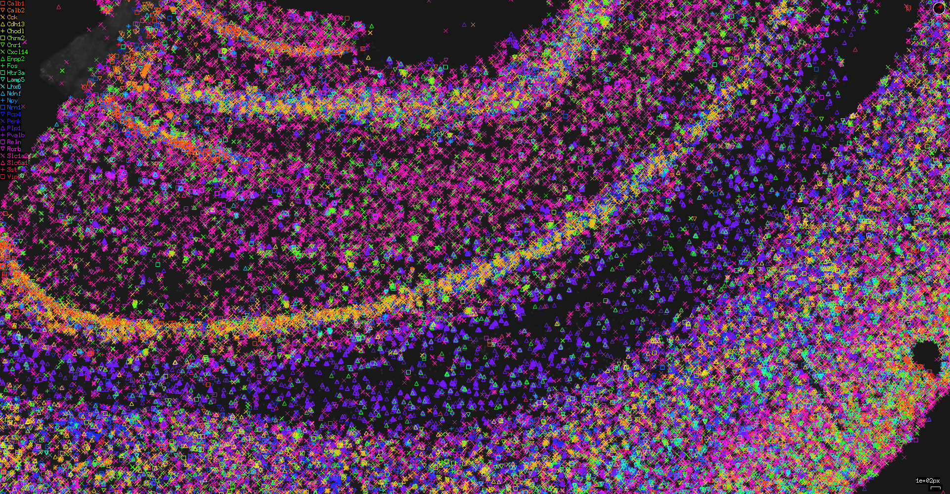
Below the collapsed sub-menus (Figure 4, B) is the “Generate network(s)” button. Pressing the button at this point will result in a network being generated using the default settings from the entire dataset. This network will appear in the network view to the right of the panel (Figure 4, D). Below the “Generate network(s)” button is the tissue view (Figure 4, C), which shows a reconstruction of the original dataset, in which each transcript type is assigned a colour and symbol.
The tissue view window (seen in Figure 5) will initially show all transcripts. Once a
network is created and some component(s) in the network are selected, the network
visualization will be filtered to show only the transcripts corresponding to those
particular nodes and edges, as described in section 3.2. All transcripts can be shown
again by selecting the show all button (eye icon):
The view can be panned by left-clicking and dragging, and zoomed at the cursor
location by moving the scroll wheel. The current zoom level is displayed to the
bottom right of the window, and below that the current coordinates of the mouse. It
is also possible to rotate the view by clicking + dragging using the third button (or
scroll wheel button). The current orientation will be updated in the compass to the
top right of the view. The legend found to the left of the view can also be
scrolled up and down (if it exceeds the height of the window) by mousing to
the far left of the view and using the scroll wheel. You may also left-click
individual transcripts to view their name. The legend, compass, scale bar, and all
other informational components may be hidden/shown using the info button:
 .
.
Often, the tissue view may be too small to provide an adequate visualization, in
which case the view can easily be popped out into its own separate window which can
then be expanded at will. To pop out the window, select the unpin button found at
the bottom-left of the panel:  . The window can later be re-pinned by
closing the window or selecting the same button (which now appears as a
pin).
. The window can later be re-pinned by
closing the window or selecting the same button (which now appears as a
pin).
The tissue view toolbar controls will follow the popped-out window. If
you wish to re-center and re-fit the zoom level, simply press the centering
button:  . This will adjust the settings to best fit the current window
size.
. This will adjust the settings to best fit the current window
size.
While exploring the tissue view, you may also wish to load corresponding
histological imagery such as hematoxylin-and-eosin (H&E) stains to assist with
navigation of the tisse. To load an image, select the image load button:  . You can
then browse to and load an image, and also optionally resize it. Most common
formats are supported, including JPG, PNG and TIFF.
. You can
then browse to and load an image, and also optionally resize it. Most common
formats are supported, including JPG, PNG and TIFF.
When components within the network are selected, the transcripts will be filtered to
only display those that correspond to the selection (provided the show all button
has not been enabled). For example, within Figure 6, no selection has been made in
the network view. But in Figure 7, the ACTB node has been selected, and this
results in only ACTB transcripts being visible in the tissue view. Notice
also that the tissue view and network view colours are matched. This is
always kept in sync, and can be adjusted from the Style control dialog (See
section
InsituNet network generation by default will use the entire imported dataset, however it also features support for network generation from any 2D subregion. This allows the user to create region-specific networks that can then later be compared and contrasted. Using the tissue view found at the bottom of the control panel, users may zoom and pan the dataset as well as manually define 2D regions using the mouse.
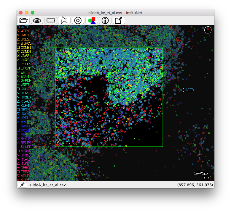
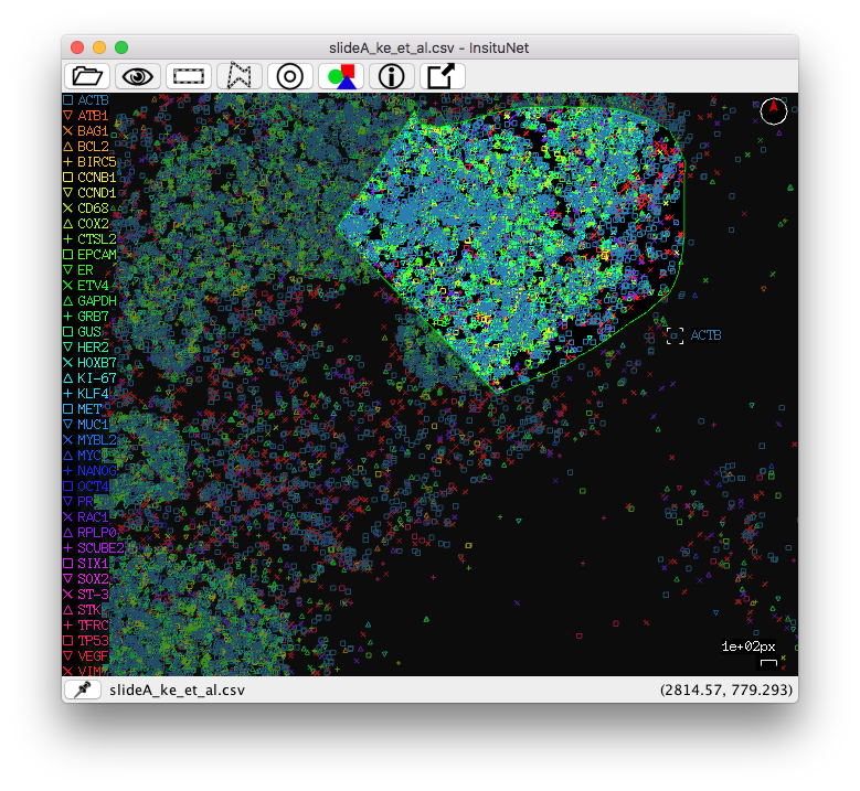
There are two modes to manualy select a specific region of the tissue of
interest, basic rectangular and freeform/polygon mode. They can be toggled
between by selecting their corresponding buttons from the tissue view toolbar:

You can select regions by using the right mouse button (or the left button while holding the control key). To select right click and hold the right mouse button until the selection is complete. Rectangular selection is simply a matter of click + drag. The freeform/polygon mode is freeform while held, but if simply clicked, a polygon point will be placed. In this mode, you will have to reconnect with the beginning of your line to complete the selection (the line appears red while incomplete, green when complete). If you have a valid selection made when the “Generate network(s)” button is pressed (and manual selection is enabled under the region selection subpanel) then the network will only be based on data in the selected region of the tissue.

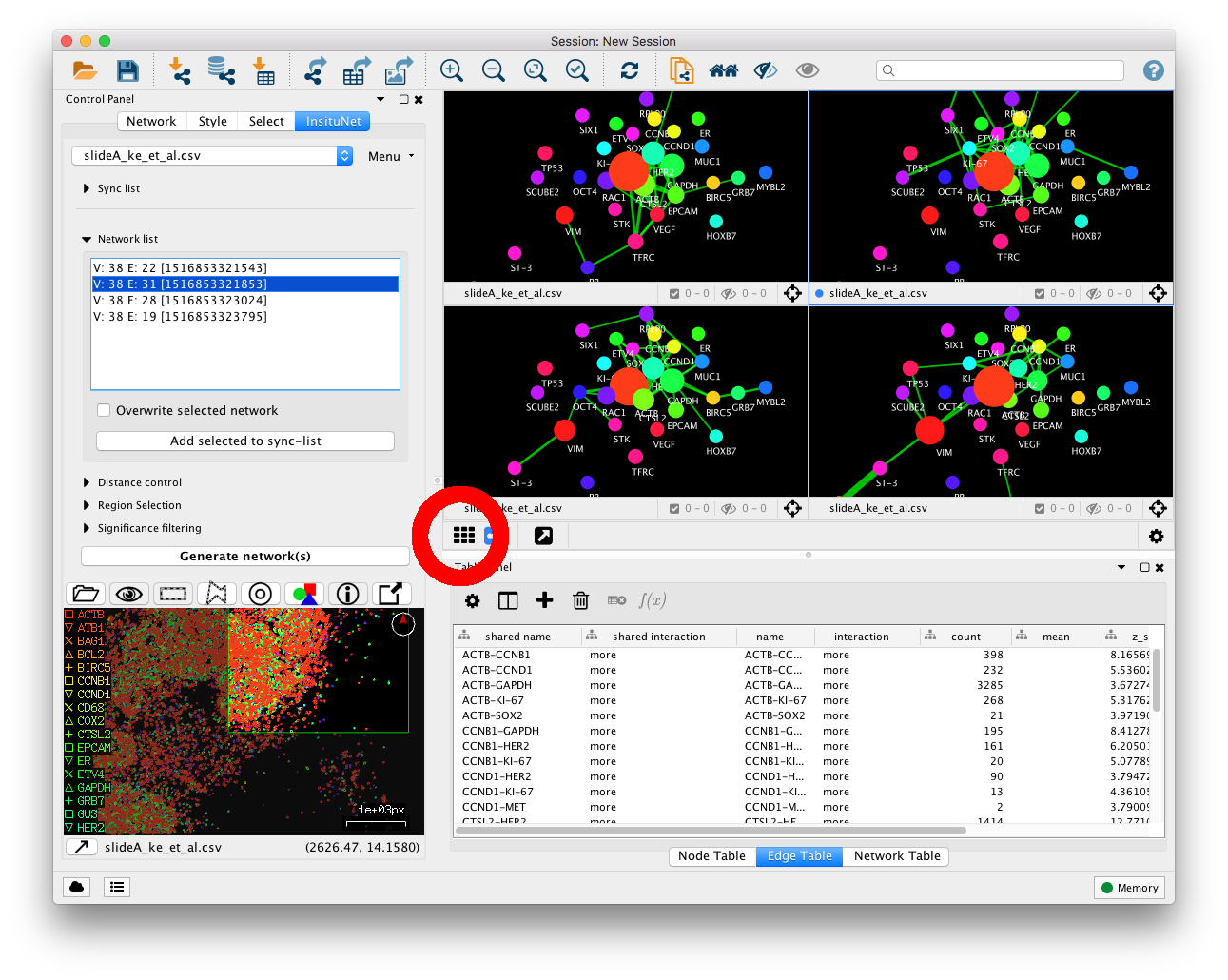
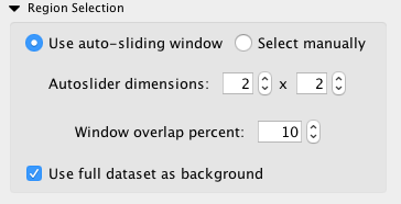
If desired, a sliding window function can be used to automatically generate networks
from a grid of rectangular selections. This option can be enabled from the region
control subpanel. Just select the dimensions of the grid (the default is a 2x2 grid,
which will create 4 individual networks). Networks will be generated in order
from left to right, top to bottom. If the selected grid is 1x1, there will be no
difference between this and using the entire dataset. On Cytoscape 3.4+,
click the grid button:  to display all the networks generated as in Figure
11.
to display all the networks generated as in Figure
11.
Each time a network is generated, InsituNet does several things. Firstly, it conducts a search around each transcript to find if they have any neighbours close enough to be considered as spatially co-expressed. Next, a network is created in which every unique transcript is represented as a node in the network. The node size is proportional to the abundance of that transcript, in relation to the total abundance of all transcripts within the selected 2D area. Details on the proportion can be found in the node table panel (Figure 4, E). Co-expressed transcripts are linked with an edge (see below for further details). Lastly, filtering is optionally applied to remove edges which are not assessed to be statistically significant, given the abundance of the transcripts. For example, if one transcript type is highly abundant and is co-expressed with almost everything, the relationship may not be of interest and can be pruned from the filtered network. There are options for filtering for relationships that occur both more and less often than statistically expected. The network created will be saved within the network list subpanel (within Figure 4, B).
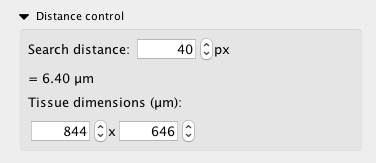
The most important variable that a user needs to define before generating networks is the spatial co-expression distance. It may be adjusted from the distance control sub-panel, as seen below.
The search distance value is given in the same units as the input file. An estimation of this value in µm is displayed below the search distance. This is estimated from the tissue section dimensions provided by the user below it. The search distance is used to determine whether any two transcripts are close enough to be considered by InsituNet as spatially co-expressed. Increasing or decreasing the search distance will result in more or fewer transcripts being identified as spatially co-expressed. Determining what the optimal distance is will depend on what your intentions are. If you are interested in looking at intracellular co-expression, you will likely want the distance to be smaller than the average diameter of the cells your data has been generated with. For example, human squamous epithelial cells are typically 40-60µm in diameter, so it would be advisable to set the search distance somewhat below 40µm.
It is also important to note that increasing the distance will increase the time InsituNet takes to identify which transcripts are co-expressed, and will likely increase the number of co-expression relationships found. It is advisable to start with a lower distance and then only increase it if needed.
InsituNet provides several methods to assess the statistical significance of spatial co-expression and to filter the network accordingly. This is to prevent the network becoming excessively dense and to focus the analysis on the most significant spatial co-expression relationships. The aim is to test whether, given the abundance of a given pair of transcripts, the amount of spatial co-expression they exhibit is surprisingly high (or low).
In situ sequencing can provide extremely dense data on the detection of 1 million or more transcripts in a given tissue section. In such dense data, we would expect to observe a large number of spatial co-expression relationships simply by chance, particularly for highly abundant transcripts. InsituNet aims to identify spatial co-expression between two transcripts that occur statistically more than expected given the abundance of the two transcripts in the data. These statistically significant interactions are more likely to represent true spatial co-expression. InsituNet can also identify transcripts that are co-expressed much less than expected given their abundance. These transcripts may represent specific biomarkers of particular cell-types or tissue regions (e.g. those associated with pathology).
Control of edge filtering is available under the “Significance filtering subpanel:
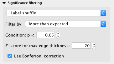
The first multi-option box defines which test will be used for the statistical analysis. This is either Label shuffle, Hypergeometric test, or no filtering.
The simplest filtering option is no filtering. This will create a network in which an edge is drawn between transcripts that exhibit any spatial co-expression at all. No assessment of significance is made. The label shuffle and hypergeometric methods are both options to assess how statistically surprising each co-expression pair is. The label shuffle method performs this by generating a distribution of values by randomly permuting transcript labels 1000 times, then re-assessing which co-expressions occur. The permution only shuffles the transcript labels/names, not their x and y positions. Significance is then determined by comparing the observed values in the real data to this distribution. The hypergeometric method is essentially the same process, except a hypergeometric distribution is automatically created rather than performing the label permutation. The default is to use to label permutation method, which generally produces good results but can occasionally rate lowly abundant transcripts that spatially co-localize extremely highly. The hypergeometric test can be less susceptible to this. By using the hypergeometric distribution, the significance of drawing k co-expressions of transcripts a and b can be assessed by fitting the following variables to the hypergeometric test parameters:
In comparison to the label permutation method, the hypergeometric test fully considers the compound probability of obtaining a certain number of co-expressions given their abundances.
The next multi-option box allows you to select whether you wish to look at spatial co-expression occurring more than expected, less than expected, or both. You can also adjust the P value threshold. Edges found to be less than the provided value will be pruned from the final network. The Z-score is used to control the maximum edge width in the network view so that the highly significant edges do not overwhelm the network visualization. The maximum edge thickness can be set to a certain Z-score, by default 20. These Z-scores and other information such as the raw transcipt counts can be found in the Cytoscape node and edge tables, which is usually found at the bottom of window (Figure 15). The final option available is to use Bonferroni correction, a method to correct for multiple testing.
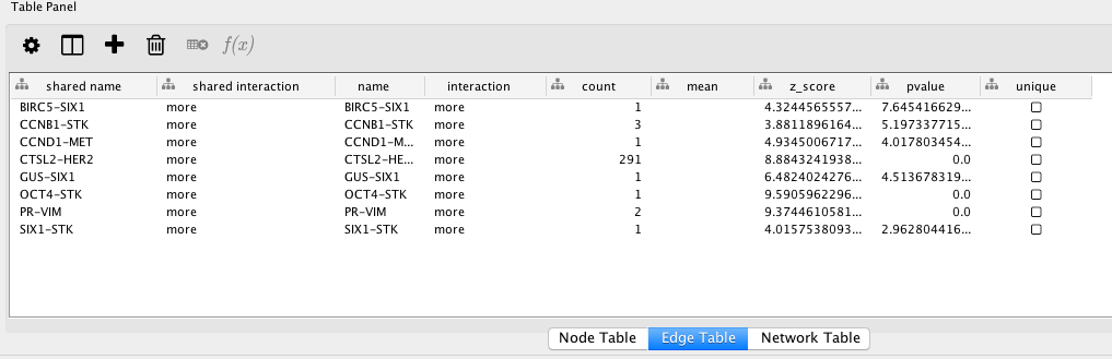
If the Table Panel is not visible, you can enable it from “View → Show Table Panel”. The node tables contain counts and proportional abundance for each unique type of transcript in the network (which is used to determine node size). The edge tables contain information pertaining to the spatial co-expression relationship that the edge represents, such as the Z-score and P value.
Networks that you have generated will appear in the “Network list” subpanel. Selecting each item on the list will automatically switch the network view to the corresponding network, and also display the region that it was created from on the tissue view. You can also use the arrow keys to quickly switch between networks in this list.
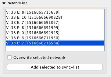
If the “Overwrite selected network” button is checked, then intead of creating a new network, the currently selected one will be overwritten. This can be useful for testing purposes, to prevent the list becoming cluttered.
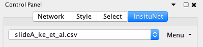
It may be desirable to compare two or more different datasets containing tissues from different locations. InsituNet allows for multiple datasets to be imported at any one time. To import a new dataset, simply go to “Apps → Import InsituNet” data and import a new file. InsituNet will automatically switch to this dataset once successfully imported, but you can switch to any previously imported datasets by using the selection box at the top of the control panel which displays the name of the current dataset:
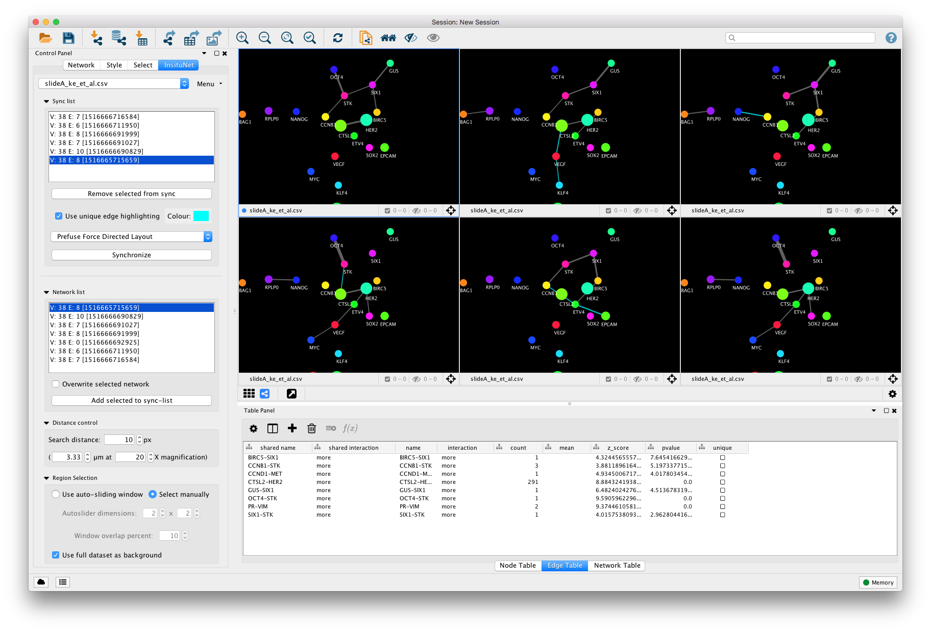
InsituNet’s synchronization allows easier comparisons between different networks (e.g. networks representing different datasets or different regions from within a single dataset). This function synchronizes the position of nodes representing the same transcripts in different visualizations, so that when switching between them it becomes easier to see which edges and nodes are altered. This is accomplished by creating an unseen union network of all synced networks, applying whatever layout is selected to the union, and then applying the position of nodes in that network to all of the synced networks. To get networks into the sync list, highlight them in the network panel then select “Add selected to sync-list”.
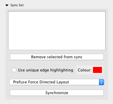
Synchronization occurs between any networks that are placed into the sync list. These networks need not be from the same dataset, either. The synchronization list is global, switching between datasets will not alter it. The synchronization is also continuous, so the layouts will stay in sync even if components are moved manually. Selecting different networks from the list will switch the view to them, as with the normal network list.
The sync list subpanel allows for selection of different layouts, and also provides options for highlighting unique edges with an adjustable colour. Unique edges are ones found in only one of the synchronized networks, and may be useful for identifying unusual associations. Selected networks may be removed with the “Remove selected from sync” button. An example of multiple synchronized networks with unique edges highlighted is presented in Figure 23. A manual Synchronize button is also provided in case desynchronization occurs for any reason (which can sometimes occur if other Cytoscape functions are used to manipulate the synchronized networks).
In these tutorials we will walk through creating and managing networks within InsituNet. We will primarily be using data from Ke et al. 2013, an in situ sequencing dataset of HER2-positive breast cancer tissue. This and other datasets such as a two-million point test dataset can be found hosted at https://bitbucket.org/insitunet/insitunet/src/master/datasets/.

You can adjust the colours of transcripts in both the tissue and network views by
using the Style control button, found above the tissue view: 
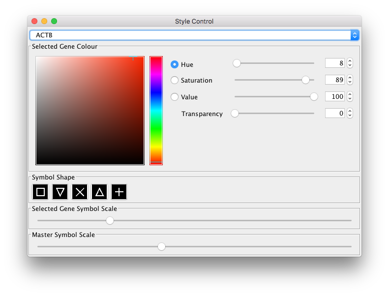
Notice that the corresponding node colours also change when you adjust the transcript colour.
You can export an image from both the tissue and network views quite easily. To export from the tissue view:

You can also choose to export with a resolution higher than the current view resolution. In this case, the center of the image will stay as the center of the window, but the height and width will be as you specify. This can be useful as it allows exporting an image larger than the screen size:
You can also export the network view using inbuilt Cytoscape functionality using “File → Export as Image...”.
All networks you generate will be listed within the Network list subpanel. However, when you import a new dataset, you will have to switch the datasets to access the Network list for that dataset, as it is local (in contrast to the global sync list).
The sliding window allows you to automatically generate multiple networks across your dataset.
Comparing multiple networks is complex, but InsituNet allows you to synchronize their layouts (and keep them in sync) to make this task easier.
Your networks are now synchronized. In later versions of Cytoscape (3.4+) you can open
these networks side-by-side and compare them all simultaneously. To do this, press
the grid button: , select all the networks you wish to view at once, then press the
view button:  . You will then be able to view multiple synced networks at
once, and see the changes update live when you move nodes or pan and
zoom.
. You will then be able to view multiple synced networks at
once, and see the changes update live when you move nodes or pan and
zoom.
The actual maximum size will vary depending on your graphics hardware. But in general it’s better to use a lower resolution image and then scale up within the program.
Some virus scanners can interfere with the way JOGL (which provides OpenGL acceleration) loads libraries at runtime. They scan everything as it loads which makes it take a long time. It should eventually load, however.
How fast this is depends on your graphics card. Idealy, use a more powerful card. There are some things that will probably increase rendering speed though, such as disabling anti-aliasing (see below) or reducing the size of points (try moving the master point scale to minimum).
By default, 2X MSAA is enabled in the tissue view, which makes transcript symbols appear less jagged but can slow performance. To disable, simply change the property insituNet.useAntiAliasing from "true" to “false” (Edit → Preferences → Properties). This will apply to any new dataset you open, and also affects the exported image.